Lab 2: Significance Testing and Chi Squared Test

Part 1 from assignment (no write up):

1.

2b: Below are all of the potential null and alternative hypotheses that could have been generated from the insects:

Null (Asian Beetle): there appears to be no difference between the number of Asian-Long Horned Beetles from the county level to the state level.

Alternative (Asian Beetle): there is a difference between the average number of Asian-Long Horned Beetles from the county level to the state level.

Null (Emerald Beetle): there appears to be no difference between the number of Emerald Beetles from the county level to the state level.

Alternative (Emerald Beetle): there is a difference between the average number of Emerald Beetles from the county level to the state level.

Null (Golden Nematode): there appears to be no difference between the number of Golden Nematodes from the county level to the state level.

Alternative (Golden Nematode): there is a difference between the average number of Golden Nematodes from the county level to the state level.

Here are the results after each z or t test:

•  I reject the null hypothesis, which states that there is a difference between the average number of Asian-Long Horned Beetles from the county level to the state level. This is because the z-score was calculated to be -7.749 and the critical value was 1.96, which does not fit into the distribution graph.

Z score: (3.2-4)/(.73/sqrt. 50)= -7.749

•  I reject the null hypothesis, which states that there is a difference between the average number of Emerald Beetles from the county level to the state level. This is because the z-score was calculated to be 9.246 and the critical value was 1.96, which does not fit into the distribution graph.

Z score: (11.7-10)/(1.3/sqrt. 50)= 9.246

•  I reject the null hypothesis which states that there is a difference between the average number of Golden Nematodes from the county level to the state level. This is because the z-score was calculated to be 2.47 and the critical value was 1.96, which does not fit into the distribution graph.

Z score: (77-75)/(5.71/sqrt. 50)= 2.46

3a:

• Null Hypothesis: There is no difference between the size of the party attending a wilderness park in 1960 and 1985.
• Alternative Hypothesis: There is a difference between the size of the party attending a wilderness park in 1960 and 1985.

T- value: (3.4-2.1)/(1.32/sqrt. 25)= 4.924

3b. The corresponding probability value is 1.711 for a two tailed 95% confidence level.

Part 2:

Introduction/ Problem/ Research Question(s):

This lab's purpose was to determine whether 'Up North' in Wisconsin is truly different from the south. In this particular situation, Highway 29 that runs from east-west was used as the dividing line between the two halves. The null hypothesis for this lab is that the 'north' and 'south' have no significant difference in their variables. The alternative hypothesis is that there is a difference between the variables in northern Wisconsin than southern Wisconsin.

Methods

The first step was determining which counties belonged on the north/south region of the state. It was difficult to find a map with both county names and Highway 29, so a county labeled map of Wisconsin was created in ArcMap and imported into Adobe Illustrator. Then a state map with Highway 29 labeled was overlayed on the other map to then be able to see the county labels, and the highway location. For counties to be considered part of the 'north' they had to have at least 50% of the county boundary above the highway (see figure 1).

Figure 1. The North-South Divide. This determination was categorized based on the county in relation to Highway 29 which runs approximately east-west in almost the middle of the state.

The data that was used for this lab was obtained from the Statewide Comprehensive Outdoor Recreation Plan (SCORP), which contained data from the DNR including license data, demographics, and other variables that would relate to the outdoors and travel.

Three variables from individual data sets were used to see if there was a statistical difference between northern and southern Wisconsin. The variables that were chosen for this particular lab include forest acerage, cottages, and campsites.

Three new fields were created within attribute table to develop a clearer visualization of the spatial distribution of the data. By looking at the 'Statistics' under the original variable columns, the maximum county number of the variable was determined. This number was then taken and divided by four, which then allowed for four sub-categories to be created. This would later allow for a choropleth map to be made as well as give the ability to export the data into SPSS (a predictive analysis software program developed by IBM).

The Chi-Square value was calculated for all of the variables in SPSS. This allows for a comparison of an observed distribution to an expected distribution of frequencies.

Results

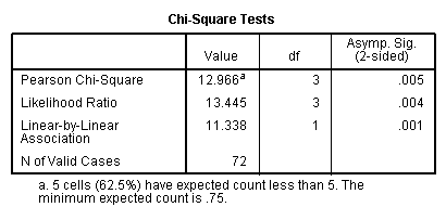
Campsites, for this dataset, are considered to be any type of campsite (see figure 2). There appears to be a fairly equal distribution of campsites throughout Wisconsin.

Figure 2. Campsites Per County.

This dataset fails to reject the null hypothesis, stating that there is not a difference between the number of campsites in northern and southern Wisconsin counties. At a 95% significance level, one would fail to reject the null hypothesis if the 'asymp sig.' is greater than .05, and because this particular 'asmp. sig.' is greater, then we fail to reject the null hypothesis (see figure 3). This is shown in the cross-tabulation table (see figure 4) which shows that there is not much of a difference between the expected and actual counts for the number of campsites. Lower central Wisconsin has the largest number of campsites in a concentrated area. It would be extremely interesting to see if there is a similar map output under the campground dataset.

Figure 3. Campsite Chi-Square.

Figure 4. Campsite Cross-tabulation.

Cottages, for this dataset, are considered seasonal homes. There are significantly more cottages in northern Wisconsin than southern Wisconsin according to the map (see figure 5).

Figure 5. Cottages Per County. 

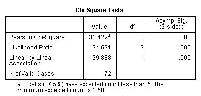
This variable rejects the null hypothesis, stating that there is a difference between the number of cottages in the north and the south because the 'asymp. sig.' is less than .05 (see figure 6). According to the map, there are statistically more cottages in the north than the south. As seen in the cross-tabulation table (figure 7), the actual counts of cottages in the north exceeds the expected in the 'more cottages' columns (columns 2-4 in figure 7), but does not hit the expected count for the 'fewer cottages' column (see column 1 in figure 7).

Figure 6. Cottage Chi-Square.

Figure 7. Cottage Cross-tabulation.

This forest data was based on public and private forested land in acres. There is an obvious trend in this data that there is more forested land in the 'north' than the south.

Figure 8. Forest Acres Per County.

The null hypothesis is rejected for this data set according to the Chi-Square Test (see figure 9). This shows that there is a significant difference between the forest acreage between northern and southern Wisconsin. This is further indicated in the cross-tabulation table (see figure 10), which shows that the county for highly forested levels was much greater in the north than the south (see column 4 in figure 10). Because the expected and actual counts were so different, there is a significant difference between the two parts of the state according to forest acreage.

Figure 9. Forest Chi-Square. 

Figure 10. Forest Cross-tabulation.

Conclusion

Overall, I reject the null hypothesis stating that there is a difference between northern and southern Wisconsin. The Chi-Square values for the forest and cottages data indicate that there is a significant difference between northern and southern Wisconsin, where as the number of campsites did not seem to have a significant difference between the north and the south. This makes it difficult when there are only three variables to draw a conclusion from, and two of those reject the null hypotheses. With different variables, we could have failed to reject the null hypothesis, stating that there is no difference between northern and southern Wisconsin.